House price prediction using Machine Learning

Today we are gonna predict price of a house just by looking at how many room, windows it has, which floor it is on, where the house located and many more factors.

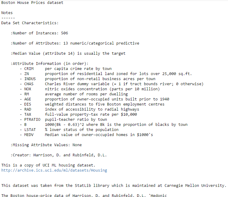
We are going to learn about implementing linear regression on Boston Housing dataset.

The Boston Housing Dataset consists of price of houses in various places in Boston. Alongside with price, the dataset also provide information such as Crime (CRIM), areas of non-retail business in the town (INDUS), the age of people who own the house (AGE). However, because we are going to use scikit-learn, we can import it right away from the scikit-learn itself.

First of all, just like what we do with any other dataset, we are going to import the Boston Housing dataset and store it in a variable called boston. To import it from scikit-learn we will need to run this snippet.

from sklearn.datasets import load_boston

boston = load_boston()

The boston variable itself is a dictionary, so we can check for its keys 

   

  print(boston.keys())

It will return statement look like this.

Available dictionary keys

Now let’s explore them.

So first of all, we can easily check for its shape by calling the boston.data.shape and it will return the size of the dataset with the column size.

    

print(boston.data.shape)

Shape of Boston dataset

As we can see it return (506, 13), that means there are 506 rows of data with 13 columns. Now we want to know what are the 13 columns. We can simply run this code and it will return the feature names.

Feature names in Boston dataset

If you are too lazy to open a web page to check the description of the dataset, since it’s available in the dataset itself then we can simply check it using this code.

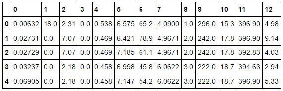
Now let’s convert it into pandas! It’s simple, just call the pd.DataFrame() method and pass the boston.data. And we can check the first 5 data with bos.head().

bos = pd.DataFrame(boston.data)

print(bos.head())

First 5 data of Boston House

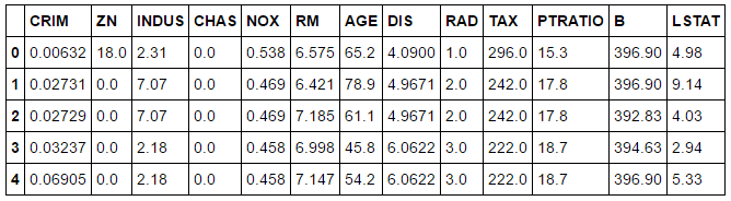
Uh, wait. Why is the column only showing its index and not its names? It turns out the column names is not directly embedded. If you remember, we have the list of the column names. So, let’s convert the index to the column names.

bos.columns = boston.feature_names

print(bos.head())

Put the feature names to the column names

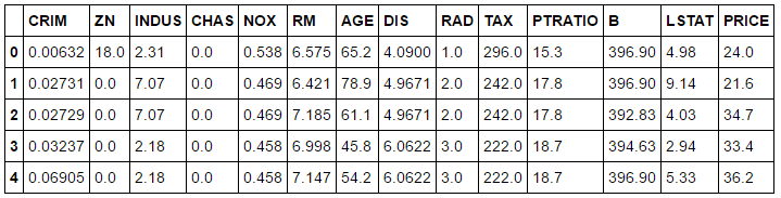
Does anyone realize that there is no column called ‘PRICE’ in the data frame? Yes, it is because the target column it’s available in other attribute called target. So let’s check the shape of the boston.target.

print(boston.target.shape)

Target shape

So, it turns out that it match the number of rows in the dataset. Let’s add it to the table.

     

bos['PRICE'] = boston.target

      print(bos.head())

                                 Data with PRICE column

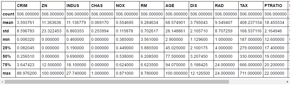
Since it’s going to be a very long post if I do all the analysis. So we are just going to the basic. We would like to see the summary statistics of the dataset by running the snippet below.

 

 

 

 

 

 

 

Split train test dataset

Unlike titanic dataset, this time we only given a single dataset. No train and test dataset. That’s fine, we can split it by our self.

Basically, before splitting the data to train-test dataset, we would need to split the dataset into two: target value and predictor values. Let’s call the target value Y and predictor values X.

Thus,

Y = Boston Housing Price

X = All other features

Now, we can finally split the dataset into train and test with the snippet below.

If we also check the shape of each variable, we can find that now we already got ourselves our train and test datasets with the proportion of 66.66% for train data and 33.33% for test data.

Shape of X_train, X_test, Y_train, and Y_test

Linear Regression

We finally going to run a linear regression. Don’t forget to import the LinearRegression.

The above snippet will fit a model based on X_train and Y_train. Now we already got the linear model, we try to predict it to the X_test and now we got the prediction values which stored into Y_pred. To visualize the differences between actual prices and predicted values we also create a scatter plot.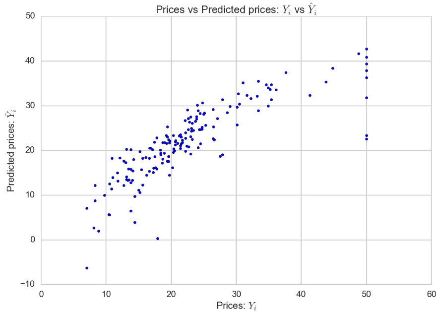

 

 

 

 

 

 

 

 

 

 

Comparison between the actual prices and predicted prices

Ideally, the scatter plot should create a linear line. Since the model does not fit 100%, the scatter plot is not creating a linear line.

Mean Squared Error

To check the level of error of a model, we can Mean Squared Error. It is one of the procedure to measures the average of the squares of error. Basically, it will check the difference between actual value and the predicted value. For the full theory, you can always search it online. To use it, we can use the mean squared error function of scikit-learn by running this snippet of code.

Mean Squared Error for the Linear Model

That means that the model isn’t a really great linear model. But, as a start, it is a good way to go. I actually still don’t understand how to know the value of acceptable mean squared error.
Thank you for being here. please comment your thought below.